MODERN PHYSICS (PHY 320) LAB

Magnetic Materials and Electromagnets

OBJECT:

To investigate some magnetic properties of matter.
To determine some properties of the magnetic fields of various permanent magnets.
To measure the  magnetic field variations of an electromagnet as a function of the coil current.
To investigate the Ising model of magnetism.
To investigate thermal demagnetization.

APPARATUS:

A set of four Neodymium-Iron-Boron disk magnets with several 1 mm plastic spacers.
A set of four Ceramic permanent magnets with several 1 mm plastic spacers.
A large Cenco electromagnet with variable gap and coils to handle currents up to 15 amps.,
associated power supply and current regulator.
F.W.Bell Gauss/Tesla Meter model 4048 for precision magnetic field measurements.
Pasco Gauss Meter and Science Workshop interface.

BACKGROUND:

In the study of magnetism and the magnetic effects associated with the motion of electric charges, one usually designates   symbols B, H, M, and µ to describe magnetic properties.

B =  the quantity known as the magnetic induction, or the magnetic flux density.  It is this property of magnetic fields that determines the force that is exerted upon a current or a moving charge.

H =  the term referred to as magnetic intensity, or field strength.  More descriptively,  it has become regarded as a
magnetizing force which acts on elementary magnets within certain material samples placed in magnetic fields.

M =  the term named the magnetic polarization or magnetization and defined as the magnetic moment per unit volume within any magnetic material.

All of the above are vector quantities.

µ = a magnetic property of matter called the permeability.  In isotropic media, it is a scalar quantity, and in many materials, like free space, it is a constant µ_o.

For most materials, the relationship between these fields can be expressed in either of two ways:

B = µ H       or    B = µ_o ( H + M)

Reference is frequently made to the example of a solenoid with some material used as the core of the windings to relate these terms.  Recall that inside the solenoid with n turns per unit length and a current I in the coil, we have approximately

B = µnI    and        H = B/µ = nI     independent of the core material.

Thus, a current in the coil produces the magnetizing force H throughout the core, and this sets up a flux density B which consists of a contribution from both the coil's field H and the material's magnetization M.  

The most easily observed of all magnetic effects is ferromagnetism, so called because of its occurrence in metallic iron and a number of iron compounds.  The experimental facts about ferromagnetic materials include that

• In these materials, very large magnetizations can be obtained.
• In these materials, M is not usually proportional to H as it is in most other materials. i.e., the value of M depends not only on the value of the applied field but also on the previous history of the sample.
• In some cases, a sample may may retain its magnetization even in the absence of of an external applied field.
• These very same materials that show such large permanent magnetization can also exist in a state with little or no net magnetization.
• In these materials, there is a strong tendency for the material to break up into many magnetic domains (regions where all dipoles are aligned), each with a different direction of magnetization, so that the macroscopic effect is to give zero magnetization.

The behavior of magnetic material during magnetization is conventionally presented as a B-H plot.

 

·         The origin of coordinates 0, represents the unmagnetized condition of a ferromagnetic sample.  When a magnetizing force is applied, the sample proceeds along the black line to point a as the magnetic polarization increases.  This line is known as the magnetization curve.

·         When the magnetizing force at point (a) is reduced, the flux density does not reduce back along the magnetization curve, but displays higher values.  When H has been reduced to zero, B still has a positive value indicated by point (b) which is known as the remanence, a measure of its retentivity. This phenomenon is known as hysteresis.

·         In order to bring B back to zero, the magnetizing force must be made negative, to a value indicated by point (c) where H has a value known as the coercive force, a measure of its coercivity.

·         When H is varied periodically about the origin the closed contour is known as a hysteresis loop.

·         The portion of the loop which lies in the second quadrant is known as the demagnetization curve.   This is the portion of interest in a discussion of permanent magnets.   In  general, it is desirable that permanent magnets have a large remanence to retain a great portion of the magnetization, and  a large coercive force in order that the magnet will not easily be demagnetized. The best single figure of merit of a permanent magnet is the maximum value of the product BH along the demagnetization curve.  Since the product BH has the dimensions of energy density, it is referred to as the energy  product and the maximum value as the maximum energy product  BH_max.

Dexter Magnetic Technologies supplies a great deal of helpful magnet background material online in their Design and Reference Manual !!! Check it out!!!

Experiment 1:    NdFeB permanent magnets

Precautions:

• These magnets should never be brought close to cassette tapes, floppy disks, bank cards, telephone cards or any other magnetic card.
• Handle carefully to prevent having a finger caught between two magnets.  This force may be great enough to cause a blood blister or an abrasion.
• When bringing two magnets together, be sure to do it slowly. Otherwise the magnets will forcibly strike each other, and chipping  of the surface may result.
• If it is difficult to separate magnets , press one against the edge of a desk and slide the other one free.

A.   Flux density versus gap length

1. Use a slotted plastic spacer to separate two magnet disks. Insert the tip of the Gauss/Tesla meter probe 1900 into the slot. Slide the probe tip along the length of the slot to find the maximum field reading.  Record it.
2. Add two spacers on either side of the slotted spacer to separate the disks and repeat the procedure.
3. Continue to add spacers one at a time and record the corresponding measurements for each different gap up to as many spacers as you have.
4. Plot B_g versus L_g.  At the Dexter Magnetic Technologies website, find the appropriate relation and fit your data to it.

B.    Flux density versus magnet volume (length)

1. Use a slotted plastic spacer to separate two magnet disks. Insert the tip of the Gauss/Tesla meter probe 1900 into the slot. Slide the probe tip along the length of the slot to find the maximum field reading.  Record it.
2. Add a third magnet disk  on one side of the pair and repeat the procedure.
3. Continue to add magnet disks one at a time and record the corresponding measurements for each different magnet length.  It may also be helpful to record the field just outside the face of a single magnet disk.
4. Plot B_g versus L_m (total length of magnets).  At the Dexter Magnetic Technologies website, find the appropriate relation and fit your data to it.

Experiment 2:    Ceramic permanent magnets

A.   Flux density versus gap length

1. Use a slotted plastic spacer to separate two magnet disks. Insert the tip of the Gauss/Tesla meter probe 1900 into the slot. Slide the probe tip along the length of the slot to find the maximum field reading.  Record it.
2. Add two spacers on either side of the slotted spacer to separate the disks and repeat the procedure.
3. Continue to add spacers one at a time and record the corresponding measurements for each different gap up to as many spacers as you have.
4. Plot B_g versus L_g.   Compare to Experiment 1.

B.    Flux density versus magnet volume (length)

1. Use a slotted plastic spacer to separate two magnet disks. Insert the tip of the Gauss/Tesla meter probe 1900 into the slot. Slide the probe tip along the length of the slot to find the maximum field reading.  Record it.
2. Add a third magnet disk  on one side of the pair and repeat the procedure.
3. Continue to add magnet disks one at a time and record the corresponding measurements for each different magnet length.  It may also be helpful to record the field just outside the face of a single magnet disk.
4. Plot B_g versus L_m (total length of magnets).  Compare to Experiment 1.

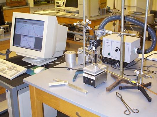
Experiment 3:     Electromagnet

   Flux density versus current:  Hysteresis

1. Zero the Pasco Gauss Meter probe in the transverse configuration away from the electromagnet.
2. Place the tip of the Gauss Meter in the center of the field of the electromagnet and record the magnitude and sign of the residual field.
3. Move the electrical connection on the Current Control box to Reverse, then measure the current necessary to zero the magnetic field, a measure of the coercivity.
4. Increase the coil current in 0.5A steps and record the meter reading until the maximum current is reached.
5. Reduce the coil current in 0.5A steps and record the meter reading.  Measure the new residual field.
6. Turn off the power supplies and move the electrical connection on the Current Control box to Reverse.
7. Repeat steps 3, 4 and 5.
8. Plot B_g versus  I, the hysteresis curve for this magnet.  Identify the retentivity and coercivity, (you will need to zoom in at values near the origin).

Experiment 4:    Ising Model of ferromagnetism

Go to the Ising model physlet found at http://webphysics.davidson.edu/Applets/ising/default.html.  Then go to the Time Development page and plot the magnetization as a function of time.

1.      Starting at T=0, find the maximum temperature at which all of the spins are aligned.  Keep B=0.

2.      Measure the hysteresis width, twice the coercivity, for T=0, 1, 2, 3, and 4.

3.      Measure and plot M vs. B for T = 0, T < T_c, and T > T_c.

4.      Using the energy plot, determine the "internal energy" or "self energy" at T=0, B=0.  What is the total energy difference between the T=0 and T = ∞ cases? (You can type in temperatures greater than the maximum value of the slider.)  What is the difference in energy between the parallel and anti-parallel spin states?  The interaction energy is given by E=Js*s. Determine J, the strength of the interaction between spins.

5.      Find the energy splitting and shift for the parallel and anti-parallel spin states for B=5.

Experiment 5:    Temperature Dependence of Irreversible Demagnetization

 Precautions:

• When handling the NdFeB permanent magnets or using the 11 kG electromagnet, be careful to keep floppy disks, bank cards, telephone cards, electronic watches, calculators, digital cameras, etc. away from the magnets.  The high field strengths may cause permanent damage to such items.
• Exercise extreme care when working around the hot plate or handling hot materials.  Temperatures in excess of 400 deg. Celsius will be reached in this experiment which can result in severe burns.

 A.  Demagnetization versus temperature

     1.      Zero the Gauss/Tesla meter probe 1900.  Find and record the maximum field reading by slowly sliding the probe tip over the NdFeB magnet.

2.      Insert the NdFeB magnet into the magnet recess of the magnet/temperature probe holder.  Check the field to see that the “Positive” pole faces up.  The temperature probe should extend about one-half of the way into the aluminum holder.

3.      Place the magnet/temperature probe holder directly on the center of the hot plate, and position the glass cup slightly above the magnet with a clamp and post fixture.  The glass cup should not touch the magnet/temperature probe holder, and the long shaft of the temperature probe should not touch the hot plate.

4.      Suspend the Pasco Gauss Meter probe into the glass cup with a clamp and post fixture, leaving a gap of about 6 mm between the end of the probe and the bottom of the inside surface of the glass cup.  The glass cup serves as a heat shield for the probe.  Switch the probe to the axial mode.

5.      Connect the large flex-hose to the air supply and suspend the 3/4 inch Tygon hose end into the cup with a clamp and post fixture, with the hose stopping about 2 cm short of the end of the probe.  Tape the hose and the field probe box together in such a way that the probe and hose are parallel to each other and parallel with the glass cup axis.  Carefully add a little length of tape around the top of the glass cup to seal the cup to the probe box, leaving an opening on the backside to act as an exhaust vent.  Be sure that the probe is centered in the glass cup just above the lowest point of curvature in the cup, and that the probe tip is directly over the magnet.  It is critical that air flows around the probe tip to cool the sensor and prevent the Hall signal from drifting erroneously.

6.      Set up your Pasco Data Studio to record Temp. versus Time, B-field versus Time, and B-field versus Temp.  Turn up the air supply blower to about the “2-o’clock” position, zero the field probe, trigger the run mode, and after about 10 seconds move the hot plate setting to position 2 (the first “on” position).  Increase the temperature setting to the next position (3, 4, 5, … ,10) every 150 seconds.  After the last temperature setting, continue to take data until 1400 seconds, and then stop the run and save your data.

7.      Examine your data.  Are the curves smooth?  How does the B-field versus Temperature compare with the “irreversible demagnetization versus temperature” curves in the TDK literature ( http://www.component.tdk.com/eneor_mg.pdf ) ?

If the B-field drifts and doesn’t level out to zero, then the probe is getting too warm and you will need to re-magnetize the magnet, adjust clearances, air flow, sealing tape and re-run your experiment. 

B.  Re-magnetization of the NdFeB permanent magnet

     1.        Gently turn on the electromagnet’s cooling water flow.  Bring the electromagnet up to full current slowly, while maintaining the current regulator’s indicator in mid-range.

2.        With the hot plate still on and the temperature reading still around 350 degrees Celsius, carefully remove the magnet/temperature probe holder.  Quickly “dump” the magnet into the long handled magnet carrier, close and tighten the cover, and place the magnet in-between the pole pieces of the electromagnet.  There is a notch on the side of the magnet carrier which indicates the location of the magnet.  Be sure to keep this mark centered between the pole pieces where the field is uniform.

3.        Keep the magnet carrier in the field for five minutes while it cools.  Then slowly turn down the electromagnet current to zero, remove the magnet carrier from between the poles, remove the magnet from the carrier, and measure its’ field with the Gauss/Tesla meter probe 1900.

4.        How does the restored field compare with your original field measurement before heating?  If it is now significantly lower, then you were probably too slow in getting the magnet into the magnet carrier and then over into the re-magnetizing field.  This must be done quickly before the magnet has time to cool down.  If the field is appreciably lower than the initial field, then re-heat the magnet to around 350 degrees Celsius holding it at that temperature until thermal equilibrium is reached, then repeat the re-magnetization procedure.