Abstract
Even though a material may have no net magnetic moment, it may acquire one when placed in an external magnetic field. As a result, a material may have an internal magnetic field which differs from the externally applied one. Important information about the physics of the material may be obtained by probing the internal field. Because an electron has an intrinsic spin and magnetic moment, it may be used as a probe of local magnetic fields on an atomic scale. From a quantum mechanical point of view, such internal field effects are manifest as spin-orbit coupling, crystal field effects, etc., which result in shifts in the electron's energy eigenvalues. An experimental technique for probing these effects is called electron spin resonance (ESR). In this experiment you use ESR to probe the local magnetic field effects in a’-diphenyl-b-picryl hydrazyl (DPPH), an aqueous solution of copper sulfate (CuSO4), and a crystal of chrome alum, KCr(SO4)2·12H2O.
Introduction
Electron Spin Resonance (ESR) provides a powerful tool for studying the unpaired electrons in condensed matter systems. In fields of a few kilogauss, the two magnetic substates of an electron differ in frequency by an amount on the order of the frequency of microwave radiation. When an incident microwave has a frequency equal to the difference frequency of two states, resonance absorption of the microwave occurs. The exact frequency of the absorption is determined not only by the external magnetic field, but by interactions with magnetic moments in the systems, which can generate local fields comparable to the external field. The proposed experiment will allow the student to observe the ESR signal for the electron spin when it is effectively free (in a sample of a’-diphenyl-b-picryl hydrazyl, DPPH), and when it is interacting (other samples).
The sample is placed in a tuned cavity, and a bridge detector is used to detect the change in reflected power from the cavity when resonance is reached. Students not only learn about the properties of ESR, but also become acquainted with the use of microwave slotted transmission lines, tuned cavities, magic-tees, bridge detectors, and AC measurements.
There are several good references which should be studied before attempting this experiment. For example, Preston and Dietz [1] have several excellent chapters on the operation of microwave waveguides, and on the experimental procedures for examining the ESR spectrum for DPPH; you should read the chapters on “Microwave Waveguide,” “Introduction to Magnetic Resonance,” and “Electron Spin Resonance.” Melissinos [2] also has an excellent section regarding the experimental setup, production of microwaves and examining the ESR spectrum in samples of CuSO4·7(H2O) and MnCl2·4(H2O); see the chapter on “Magnetic Resonance Experiments.” Microwave components are described in the book Microwave Engineering, by Pozar [3]. The method for growing a crystal of chrome alum is presented in the book Crystals and Crystal Growing, by Holden and Morrison [4]. A thorough discussion on AC measurements and lock-in amplifiers may be found in the text by Horowitz and Hill [5] and the article by Coor [6].
The first goal of the experiment is to measure the Lande g factor for the organic salt DPPH (diphenyl-picryl-hydrazyl, (C6H5)2N-NC6H2 (NO2)3), which has a very strong and narrow line, with a g factor very close to the value for free electrons. You should also consider verifying some of the theoretical equations. For example, using the DPPH sample, you should be able to verify the dependence of the resonant magnetic field on the microwave frequency. The width of the resonant peak should also provide valuable information regarding the local environment of the electron. You should also be able to understand the experimental instrumentation, such as how a lock-in amplifier operates and how the microwave spectrometer works.
The following sections provide a detailed description of the apparatus and the procedure for finding the ESR signal. There are questions which you should be prepared to answer in either the oral talks or in the lab report.
Experimental Apparatus
Electromagnets and Power Supplies
10mW Gunn Diode Oscillator or 100mW Gunn Diode Oscillator and Power Supply
Microwave System
Audio Frequency Power Amplifier
Computer with data acquisition system
DPPH sample
The experimental apparatus consists of a large electromagnet with its power supply, a set of Helmholtz coils with a ramping power supply, a 100mW Gunn diode oscillator and its power supply, a microwave system (waveguides, ferrite isolator, directional coupler, frequency meter, detector with tuning stub, variable attenuators, magic-T, crystal detector, phase shifter), gaussmeter, lock-in amplifier, audio frequency power amplifier, computer with data acquisition system, and DPPH sample (kept in freezer). Some of these are discussed in the paragraphs below; an illustration of the microwave system is presented in Fig. 1.
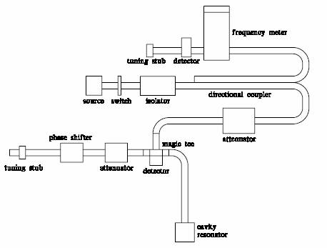
Figure 1. Schematic of the microwave apparatus.
Oscilloscope If you want to look at a signal which has a 5V DC level about which oscillates a 20mV signal at some frequency, you need to know how to use the oscilloscope effectively. Simply placing the oscilloscope on AC with a sensitivity of l0mV per division will only show the 20mV oscillation and no information about the 5V DC offset will be present (nor any indication that it is even there). This is because on the AC setting the oscilloscope automatically removes any DC offset voltage. To see this DC offset voltage you would need to set the input for DC and the sensitivity appropriate for 5V. However, here you will not see the 20mV AC signal since its size is too small compared to the 5V signal. Also, if the signal were a 5V DC offset with a 2V oscillation, the DC setting will show both whereas the AC setting won't. Thus, when both the AC and DC component of a voltage are needed, you must know how to look for them.
Waveguide A waveguide is a hollow single conductor, of rectangular cross-section for our setup. Preston and Dietz have solved Maxwell's Equations for the electric and magnetic fields in the rectangular metal walls of the waveguide and in the dielectric (air) inside the guide. They also suggest a method to determine the “cutoff” frequency, the lowest frequency which will propagate in the waveguide.
Gunn Diode The Gunn diode (MDT MO87149-2 100mW Transceiver or MaCom MA87728-MO1 10mW Transceiver) is the microwave frequency signal generator which operates on a 9V power supply (8V if the 100mW unit is replaced with a 10mW unit). Do not operate the transceivers at a higher voltage than rated, or else the unit may be damaged. The frequency of the microwaves is factory set. Generally, the power emitted by a typical Gunn diode for ESR experimentation is of the order of 5-10mW, although with the use of a 100mW unit the resonance signal is considerably easier to find and observe. Note that the 100mW unit operates at a good fraction of an Ampere, and heats up significantly with time (this is normal).
Following the Gunn diode is a waveguide switch, and then a ferrite attenuator. This ferrite attenuator serves one important purpose: to isolate the waveguide from the source. As the “load” on the Gunn diode source changes, (such as placing the sample in the resonant cavity, or more importantly, adjusting the magnetic field for ESR resonance, i.e., absorbing more of the microwave energy in the sample itself), this will change the impedance characteristics of the sample cavity, and therefore would change the impedance seen by the Gunn diode source at the other end of the waveguide. By placing the ferrite attenuator between the source and the waveguide, the coupling between the source and the load is reduced so that the operation of the Gunn diode is not greatly affected by changes in the load conditions. Usually so called “unidirectional devices,” such as this ferrite attenuator, are superior for isolation without a great loss in the transmitted power from the source to the waveguide.
Resonant cavities Two resonant cavities are used in this experiment. The first is a “wavemeter” and is used for measuring the microwave frequency. The other is the sample chamber, and will contain the sample being studied. While there is a detailed theory regarding the use of resonant cavities and waveguides, the following summary should be sufficient for you to understand the measurement of the microwave frequency. We all know that it is possible by blowing across the top of a soda bottle to excite a resonant frequency in the bottle and that one can change the frequency by adding water to the bottle. This is completely analogous to the microwave wavemeter. However, here we are interested in the amount of energy that gets transmitted past the resonant cavity. Suppose, for example, that the microwave frequency is far from those for the resonant frequency. Then it is difficult to excite those natural frequencies of the resonant cavity and all the energy will be transmitted further down the waveguide. In contrast, think what will occur when the frequency of the microwaves in the waveguide matches the resonant frequency of the cavity. Now some of the energy in the microwave field can excite resonances in the cavity and less energy will be transmitted past the resonant cavity. Thus, it is possible to measure the resonant frequencies of a resonant cavity by monitoring the intensity of the transmitted microwaves as a function of frequency. Resonances of the cavity will appear as dips in the output of the detector. In our system, instead of changing the microwave frequencies with a fixed resonant cavity, we will change the size of the resonant cavity to measure the frequency of the microwaves produced by the Gunn diode. Thus we will monitor the signal, using the oscilloscope, from the diode detector located on the wave guide tuning stub after the HP wavemeter. The cavity size is then changed by turning the adjustment and watching for a change in the DC level on the oscilloscope. A sharp dip corresponds to the resonant frequency for the cavity and the frequency can then be read off the pre-calibrated dial. We want resonance in the other resonant cavity so that a maximum power can be transmitted to the sample that is placed in it. This cavity also has some coil windings for small signal modulation of the magnetic field which will be discussed later. The nominal resonance frequency for the sample cavity should be near 9.5 GHz. Note that the sample cavity also has an adjustment of the opening size, controlled by a Teflon screw reachable from the back of the magnet. This can be adjusted for maximum effect at the crystal detector of disturbance inside the chamber (e.g. by wiggling the sample around a bit).
Attenuators, phase shifters An attenuator attenuates (decreases) the power traveling through it without changing the frequency. A phase shifter does just what its name implies; it can be used as an attenuator by combining a reflected wave out of phase with the source wave. The system also contains tuning stubs which adjust the length of the waveguide and thus will change the characteristics of the reflected wave.
Diode Detector The microwave detector is the commonly used “crystal diode,” which consists of a silicon crystal in contact with a fine tungsten wire, known as a “cat's whisker.” In certain regimes, the DC voltage output of the detector circuit is proportional to the incident microwave power. As discussed below, we will be using the detector to measure the relative power rather than the absolute power. However, you should use the attenuator to measure the relative sensitivity of the diode detector (i.e., change the attenuator by x dB and monitor the change in the output of the diode detector).
Magic-T The heart of the microwave spectrometer is the bridge circuit, and its primary component is the “magic-T.” One important reason to use a bridge circuit in the spectrometer is for sensitivity. For example, as discussed later, the output of the diode detector, which is located in the front of the spectrometer, is usually on the order of hundreds of millivolt. However, the ESR signal may be on the order of a few millivolt. Thus it may be rather diffcult to see the ESR signal riding on top of this hundreds of millivolt signal. Two important techniques to increase the sensitivity of the spectrometer are used in this experiment. First, we use a bridge circuit which adds some additional complexity to the circuit but allows one to zero out this hundreds of millivolt signal for greater sensitivity. Secondly, as discussed below, we will modulate the magnetic field by adding a small AC component, which will result in an AC modulated ESR signal, which can be input into a lock-in amplifier.
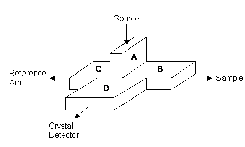
Figure 2. Schematic of the magic-T.
The magic-T is a four port device shown in Fig. 2, with some very special properties. Let's assume that the microwave power is flowing in from port A. One might assume that this microwave energy will be equally divided between ports B, C and D. However due to the different polarizations of the electromagnetic field and the configuration of the slots leading to the four arms, the power is not equally divided between ports B, C, and D. The microwave power flowing in from port A can branch into B and C but not into D. On the other hand, power which flows back, (reflected) from B and C can flow into D and is split equally between A and D. Therefore if we can match the power flowing back from ports B and C, they will superimpose at D to give a null output. Thus in this spectrometer, we will have the sample arm of the bridge off port B and a reference arm off port C. By adding phase shifters and attenuators in the reference arm, we can match the impedance of arm C with that of the arm off port B which contains the sample. Therefore, as long as the arms are balanced and the magnetic field is far from the ESR resonance, the output of the detector located on port D will be zero. However, at the proper setting of the magnetic field corresponding to the electron spin resonance, the arms will no longer be balanced, as microwave energy is absorbed by the sample and there will be a non-zero signal from the detector at port D.
Magnets The ESR system utilizes three electromagnets. The primary magnet will be used to produce a field on the order of a few kilogauss. This will require a source current capable of producing a large amount of heat in the magnet over a period of time, and therefore the magnet must be water cooled. The water flow must be on at all times when the primary magnet is in use and checked periodically for temperature rise during use. Monitor the water connections for possible leaks. The secondary magnet is smaller and consists of Helmholtz coils found between the two sides of the primary magnet. The Helmholtz coils will be used for producing fields up to about one hundred gauss. The third source of magnetic fields is the set of coils in the sample cavity which will be used for the production of a few tenths of a gauss.
Power supplies There are three power supplies used in this experiment. One powers up the Gunn diode. Another is a small homemade power supply which will power the secondary magnet; this power supply has built-in voltage ramping (either up or down) circuitry, with a ramp rate and amplitude controlled by knobs on the front. The third power supply (HP 6030A) is relatively large, and is used for the primary magnet. The large power supply is capable of producing fairly high voltages (over 50 volt) and large currents (of the order of several ampere) and should be treated with caution. NOTE: Be sure that the cooling water is flowing through the magnet prior to turning on the large HP power supply; an interlock switch is employed to ensure this. Also periodically touch the sides of the large magnetic windings to make sure that the magnet windings are not heating up due to some blockage in the cooling water hoses. NOTE: When powering up the primary magnets a very large change in magnetic field strength will occur with relatively small changes in the voltage due to the large number of windings in the magnet. Since there exists a reversing induced voltage (due to Lenz's Law), which goes as the inductance times the time-rate-of-change of the current, the power supply will be forced to push against it to maintain its voltage as the current changes. Therefore the voltage (or current) must be increased or decreased slowly so as not to cause a surge through the power supply.
Hall Probe and Gaussmeter The Hall probe gaussmeter (F.W. Bell Series 9900 gaussmeter) is used to measure the field near the cavity containing the sample. The probe is a delicate instrument and must be handled with care. The orientation of the probe should be such that the surface area of the flat sides intersects as many field lines as possible so as to get the maximum reading possible. The gaussmeter should have a reference manual with it and this manual will be of much more value than any explanation here. Basically, the meter measures the magnetic field via the Hall probe. The meter has several functions making use of relative readings, absolute readings, scale or range, units of measurement, and more. The unit also has a GPIB interface for computer sampling of measured field.
Lock-in Amplifier (What is, Frequency Domain, EG&G Princeton Applied Research Model 5209 Lock-in Amplifier)
The lock-in amplifier is used to extract low-level signals from noise. Measurements of DC voltages are sometimes complicated by the pickup of noise from the environment; at low frequencies noise is inversely proportional to frequency, so the noise is worst at DC. While there are methods to average out the noise by signal averaging over some time period, it is much better to modulate some parameter in the system and thus shift the measurement to a higher frequency where there is less noise; this is the motivation for an AC measurement technique [5, 6]. In the ESR experiment we will modulate the magnetic field by a small amount as a function of time, so that the total field is B0 + Bmod cos(wmodt) ; and use the lock-in to monitor the changes at that modulation frequency. If the frequency of this additional magnetic field Bmod cos(wmodt) is slow compared to the GHz frequencies of the microwaves, then the total magnetic field changes so slowly that we can consider it to be “quasi-static.” Typically, we will use a modulation frequency of around 200Hz, 106 times slower than the microwave frequencies. By modulating the signal, we will ultimately be measuring the slope of the ESR resonance curve [5]. Provided that the overall amplitude of this time varying field is small, your data plot will be a picture of the first derivative of the ESR signal with respect to the magnetic field.
Power Amplifier The power amplifier (Krohn Hite Wide Band DC-1MHz 10 Watt Amplifier) is used to amplify the drive modulation signal from the lock-in to the probe coils. It acts only as a power amplifier to amplify the current and does not change the voltage. This is to avoid damaging the lock-in amplifier by attempting to draw too much current out of it; the power amplifier works in the same manner as a voltage follower.
Computer The computer will be used in conjunction with several other pieces of equipment for scanning a small increment in magnetic field strength and recording the data. For every incremental change in output voltage from the homemade power supply, the computer will read the value of the magnetic field and the value of the lock-in amplifier output and then display the results using a LabView Virtual Instrument (VI), allowing the writing of the data to a file.
Procedure
1. Initial set up.
(a) Zero the gaussmeter according to instructions in the manual.
(b) Place some DPPH in the sample tube to fill a length of about 1 cm, and place some nonconducting material into the sample tube to allow the sample material to be concentrated into one location. Note that DPPH is supposed to be stored at freezing temperatures, so that you may have to look in the lab's freezer for the sample.
(c) Place the Hall probe as near as possible to where the sample will be located (usually just outside the cavity). You will have to carefully determine how the magnetic field outside correlates with the magnetic field inside, and correct your measurements for the difference.
2. Tuning the microwave system is as follows:
(a) Set the voltage on the Gunn diode to 9.0 V for the 100 mW unit (8V for the 10 mW units).
(b) Place the sample into the sample cavity. The sample must be located in the center 1/4 to 1/2 of the waveguide.
(c) Set the reference arm attenuator to maximum attenuation to decouple it from the system. Reading off the signal at the magic-T (~50 mV for the 10 mW unit, ~500 mV for the 100 mW unit), vary the Gunn diode frequency (small screw adjustment) until a minimum amplitude (i.e., closest to ground) signal is seen; note the many frequencies at which minima are seen, corresponding to various resonance modes of the sample cavity; use the mode with the lowest resonance magic-T signal. Measure the frequency at the measurement cavity. (Note: many modes seem to have about the same lowest magic-T signal; the nominal resonance frequency of the cavity is about 9.54 GHz).
(d) Measure the signal at the magic-T on the oscilloscope and adjust the setting on the attenuator on the reference arm and/or on the setting of the phase shifter until a minimum is achieved. Such a minimum in signal strength corresponds to a resonance in the sample resonant cavity; thus the spectrometer will be tuned for the greatest sensitivity for observing the ESR signal. Repeat adjustments until the signal being detected is the smallest signal attainable, which means that all (or as much as possible) of the signal is being resonated in the sample cavity.
(e) Shift the position of the DPPH sample. You should see a fairly large (tens of mV) shift in the baseline of the diode output as you shift the position of the DPPH in the resonant cavity. This will ensure the proper positioning of the sample in the resonant cavity. You may have to adjust the opening size of the cavity via the Teflon screw on the back of the resonant cavity to maximize the response at the magic-T to disturbances in the cavity (e.g. wiggling the sample around a bit). NOTE: you may have to return to step (c) and readjust the microwave frequency if the sample needed a large readjustment in position.
(f) Balance the bridge by adjusting the phase shifter, attenuator, and wave guide length adjuster to attain a minimum signal on the 5mV scale on the oscilloscope (can be zero for the 10 mW unit, about 20 mV for the 100 mW unit). In most cases, one should be able to balance the bridge with just the phase shifter and the attenuator. The best method is to adjust the attenuator to minimize the signal and then adjust the phase shifter. By readjusting one device, leaving the other fixed, you should be able to zero out the bridge in three or four repetitions.
(g) Offset the signal by a small amount to ensure that the detector diode is on and will respond to small changes in power. Usually a shift on the order of 10-20mV is sufficient. For the 100mW unit, it is likely that no additional offset will be needed.
3. Bring magnetic field up to expected range as follows:
(a) Calculate the expected magnetic field.
(b) Power up the primary coils with the HP power supply to within 30 G of the expected value. Remember to account for a possible offset between the magnetic field measured just outside the cavity and the one of interest inside the cavity!
(c) Monitor the signal at the magic-T and slowly sweep the magnetic field by means of the secondary coils and the homemade power supply. The ESR resonance should show up as a change in the DC level of the signal. The change is ~1mV for the 10mW unit, ~10mV for the 100mW unit. NOTE: the size of this signal will depend on the rate at which you are ramping the magnetic field; sometimes it will appear as a sharp “blip” on the oscilloscope. If no “blip” on the oscilloscope is seen, then check calculations, wiring, sample, etc. or try sweeping a different range of field.
(d) Once the resonant field is found, turn off the secondary coils and adjust the primary coils to approximately 20G below this peak.
(e) Set the gaussmeter to read relative to this field and record the relative offset value in your data notebook.
(f) Adjust the primary coils to within 10G of the peak. The relative gaussmeter reading should be on the order of 10G now.
(g) Determine the range of voltages provided by the homemade power supply to the secondary magnet coils that result in a magnetic field total sweep of about 20G. In step 4, we will scan from 10G below resonance to 10G above.
(h) Understand the gaussmeter output by monitoring on a scope the DC analog signal from the back of the gaussmeter as you slowly change the magnetic field by changing the signal from the homemade power supply.
4. Set up the lock-in amplifier as follows:
(a) Connect the magic-T to the “A” input on the lock-in amplifier.
(b) Connect the “Reference osc” signal out of the lock-in to the input on the Krohn Hite amplifier, which is located on the back of the unit.
(c) Connect the Krohn Hite signal out to the modulating coils at the sample cavity. The signal out is located on the front of the amplifier. Keep the Krohn Hite amplifier to a setting of ×1CPS; in this setting, the adjustable gain knob is irrelevant.
(d) One important parameter you need to control is the size of the modulating B field. If it is too large, then it will be difficult to see the ESR signal. One method to set this field is the following. First, set the frequency of the lock-in to around 20 or 30Hz. Set the Osc Level to 1.0V. Determine the peak-to-peak change in magnetic field by observing the peak-to-peak change (back of the gaussmeter) in mV on the oscilloscope. Do this for different Osc Levels.
(e) Assuming that the peak width of the ESR resonance is of the order of the range of magnetic field we will be sweeping (20G), calculate the size of the modulation signal which would yield a modulated sweep of 1/100 of the total sweep (i.e., total sweep = 20G, modulated sweep = 20/100 = 0.2G). This way only a small part of the curve will be looked at when measuring the slope. Use the Reference osc settings to set the appropriate output voltage for the calculated modulation signal. Disconnect the analog output of the gaussmeter and return to monitoring the output signal of the diode detector.
(f) Set the lock-in modulation frequency such that you will not pick up noise from any nearby electrical appliances (i.e., not a multiple of 60Hz). Usually a frequency around 200Hz is fine.
(g) You can check the sensitivity setting of the lock-in amplifier by slowly ramping the field up to the appropriate ESR resonance field strength. You should be able to observe the ESR signal on the scope as a small AC signal of the same frequency as the lock-in setting. If the modulation amplitude is large, you might see two blips per lock-in cycle, as the magnetic field sweeps past resonance twice per cycle. This is sometimes easier to observe if you trigger the scope off the output signal of the lock-in. If the resonance signal looks asymmetric, adjust the phase of the bridge balance circuit slightly. If everything is ok, ramp the magnetic field down to the previous value of about 10 G below the ESR peak.
(h) Set the lock-in time constant such that the noise on the display is averaged over to give a fairly constant value. A setting of 1s or 300ms should suffice.
(i) Set the sensitivity on the lock- in amplifier. After a trial run the sensitivity can be adjusted to make use of the full scale or to eliminate going off-scale. A sensitivity of 30μV might work.
(j) You can sweep the 20G range with the homemade power supply and monitor the output of the lock-in. Verify that a large response is observed as the magnetic field sweeps past the ESR resonance. If the lock-in’s response is saturated, adjust the sensitivity level.
5. Use the computer to display the lock-in response and store the data as the magnetic field sweeps over the 20G range.
(a) Run LabView, and load the ESR_gmdirect.vi VI (Virtual Instrument) to display and store the readings from the gaussmeter and the lock-in amplifier.
(b) The parameters that are input to the VI are:
Drive Output, Volts: enter here the Reference osc voltage level driving the coil inside the resonance cavity.
Coil Calibration, Gauss/Volt: enter here the calibration determined in 4.(d) above, i.e., the signal inside the coil induced by the lock-in’s reference oscillator output signal.
Number of Readings: this is the number of readings over which each measurement is averaged; a number between 10 and 20 should work.
Gaussmeter offset, Gauss: this is the magnetic field used as a reference in the “probe relative” mode of the gaussmeter; this is displayed on the gaussmeter readout.
Gaussmeter range multiplier: automatically determined by the software: number of G per V from the gaussmeter.
Note: in plotting dV/dB vs B, only the B axis needs to be carefully determined; the dV/dB axis can be in arbitrary units. The Drive Output and Coil Calibration fields only affect the vertical scaling of dV/dB, so that really any values of these fields that do not affect the execution of the VI are acceptable.
(c) If the dV/dB vs B curve is not symmetric, adjust the phase of the bridge balance circuit slightly.
(d) Remember to write down the lock-in amplifier settings, and the relative probe offset for the gaussmeter for all final runs. Also record the microwave frequency. Remember to correct the magnetic field outside the cavity to the one inside.
Theory Questions
1. What is the magnetic moment of free electrons?
2. What is the Lande g factor? Why is it needed? Why is g not exactly two for a free electron?
3. How does g depend on the environment of the electron?
4. If the magnetic moment of the electron is aligned along the z-axis with no external magnetic field, describe the effect of turning on an external magnetic field aligned along the x-axis.
5. What are the Larmor frequency and the gyromagnetic ratio?
6. Show that for a free electron in a 5kG magnetic field the Larmor frequency is 14 GHz.
7. Why are microwaves necessary to study the electron spin resonances?
8. How do microwaves differ from light?
9. What is the quantum mechanical coupling probed by ESR?
10. What selection rules are important in determining the experimental frequency and/or the magnetic field? and why?
11. Do you expect the resonance frequency to change if the sample is changed?
Experimental Questions
1. Describe the measurement circuit used in the experiment.
2. What is a Gunn diode?
3. How is the microwave frequency measured?
4. What is a magic-T?
5. Why does the spectrometer use a bridge technique?
6. How does a lock-in amplifier work?
7. What advantages does the AC technique have over a simple amplitude measurement?
8. How does a gaussmeter work? Why is the probe so sensitive to orientation?
9. How is the magnetic field controlled?
10. Why is the DPPH sample so useful in calibrating the spectrometer?
11. Would it be possible to perform the experiment by sweeping the microwave frequency with the field held constant, instead of the current method of scanning the magnetic field with a fixed microwave frequency?
12. What would be the resonance response for free electrons? How is it different than the response for DPPH?
13. How should the strength of the resonance line depend on sample volume and density?
14. Can you make any estimation of the linewidth of DPPH? How should these be related to the spin-spin relaxation time T2?
References
[1] D. W. Preston and E. R. Dietz, The Art of Experimental Physics, Wiley, New York (1985).
[2] A. C. Melissinos, Experiments in Modern Physics, Academic Press, Orlando (1966).
[3] D. M. Pozar, Microwave Engineering, John Wiley & Sons, New York (1998).
[4] A. Holden and P. Morrison, Crystals and Crystal Growing, MIT Press, Cambridge (1982).
[5] P. Horowitz and W. Hill, The Art of Electronics, Cambridge University Press, Cambridge (1980).
[6] T. Coor, J. Chem. Ed., 45, A533 and A583 (1968). “Signal to noise optimization in
chemistry.”