"Demons in Physics"

An Introductory Lecture on the Theory of Errors and Fluctuations

in Experimental Physics

Professor J. A. Golovchenko

Harvard University

(first draft)

There are many motivations that drive people to perform experiments. Sometimes it is because you will simply need to know the value of a physical quantity to build something. If you become a good experimental physicist you will be designing and building scientific equipment to measure some new thing or some old thing in a new way all the time. You will be standing on the shoulders of a great many other people who have determined and recorded for you the numbers that describe the physical properties of matter (density, strength, thermal conductivity, electrical resistance, heat capacity, etc. etc.) that you will need to know to get anything nontrivial to work right. If you can't find a number, you'll have to figure out how to measure it yourself. Besides using this number to build your own gadget you will ultimately want to let others know your result as well.

Perhaps you are doing an experiment to probe nature because you want to "understand" something better. Often this means that you are searching for, or testing, a simple mathematical model of reality, which together with some words of explanation, constitute what most physicists call a theory. Successful theories are those that are simple and accurately predict how matter and the various other forms of energy behave under various circumstances. They are highly prized intellectual objects because they help predict the numbers we need to build things and they provide a conceptual framework to think about all those controllable and sometimes uncontrollable things that go on around us all the time. When we understand things we feel better and we might even be more useful.

So what does all this have to do with "error analysis". Well ultimately the outcome of all experiments is a number or a collection of numbers, and whether we use them to build something or understand the world around us, their value to us depends on how accurately we know them. Clearly you can conclude that one reason for studying "error analysis" is to understand the accuracy of the numbers you are using or producing and maybe even help provide guidance to produce more accurate numbers.

This is all true and very important. There is another reason for studying the subject however which is often overlooked or not stated. It is that as you attempt to obtain more and more accurate numbers by probing nature with more and more delicate equipment you invariably discover that fundamental physical processes are at work whose consequences are to contribute uncertainty to the numbers you are trying to determine. These processes are as an important part of nature as any other and learning how understand them, to live with them, to overcome them or use them is an essential part of being a physicist. Ultimately the "errors" and fluctuations in nature are controlled by the fundamental quantum mechanical structure of the world and the way in which the various forms of excitation energy are distributed and transported. It's always important to know the ultimate limits. With this bit of motivation we begin our elementary discussion.

Imagine you have carefully set up an experiment to measure a single number that perhaps characterizes matter (e.g.. the mass of an electron) or perhaps characterizes the outcome of some dynamic situation (the time it takes for a sodium atom to fall one centimeter from rest in a vacuum chamber). Lets call the property or quantity we have determined to measure A. Make a measurement and get an answer. In our imaginary experiment we shall assume we get

Now imagine that a brilliant theoretical physicist has just published her theory of "A" in Physical Review Letters and for the conditions of the experiment it predicts

.

Something is wrong. Is it with the theory or experiment? Do the experiment again. Get

.

What's wrong. You do the experiment over and over again and the value you get for A just keeps jiggling around. You do your best to improve the experiment but inevitably the value of A keeps changing. Being a physicist you decide to create a model for what's going on. Here it is.

The experiment proceeds along flawlessly and produces the "correct" value for A

.

but before that number gets to you it is changed by a "demon" to

where e is a positive or negative number chosen by the demon. Every time we redo the experiment the demon uses another value of e to confuse us. The demon is of course some aspect of the physics and reality that we do not yet understand. Lets make a model for the demon. We won't make it too simple and our results will be quite interesting as you shall see.

Imagine that our demon is equipped with a function e(g) which he uses to decide which value of e he will use in a particular experiment to fool us. We assume that g can only take on values between zero and one. In any particular experiment the demon picks a random number between zero and one, calculates the value of e with e(g) and adds this to the "correct value" of A. The kind of function we have in mind for e(g) is shown in figure(1), below

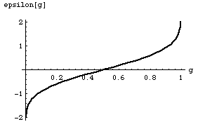
Figure(1)

We will be more concerned with calculating probabilities from e values and hence the inverse function g(e) plays the important role for us. It is shown in figure (2).

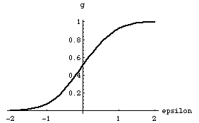
Figure(2)

Now if we insert a value for e into this function it produces the particular random value of g with which it is associated. More interestingly though is the fact that if we assume that the random numbers g that the demon picks are uniformly distributed, i.e. none is more likely to be picked than another, this will not be true for e. In fact since the probability of picking a g value between g and g+dg is just dg the probability for picking an e value between e and e+de must be (dg/de)de which is the same as dg. Thus regions where dg/de is large will lead to large probability densities dg/de in e. dg/de is such an important function to us that we will give it a new name f(e). It is the first probability density distribution in this lecture so lets describe exactly what it means and how it is used. f(e) is defined so that

This kind of dancing around is necessary because e is taken to be a continuous variable. Based on its definition f(e) will be normalized in the sense that

This follows from the fact that the range of the random variable g was chosen to be between zero and one. A particular function f(e), consistent with those shown in figures(1) and (2) is shown in figure(3).

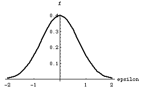
Figure (3)

The normalization requirement on f(e) is physically reasonable for it states that with unit probability, i.e. with certainty, the demon will pick some e.

In order to see how we use this distribution function we must introduce one more distribution function which will be called P(A') which is defined so that

We require that P(A') be normalized as an acceptable probability should be.

The function P(A') must represent the probability density that would be deduced for the value of A if many measurements on the same system were performed so that all random variables were sampled. This of course can never be done since it would require an infinite number of experiments for a continuous random variable. It might be better to call it a limiting probability density distribution therefore, but it's already a mouthful to say. At any rate, the concept of probability as an experimental quantity involves the use of such limiting concepts which should be familiar to students of physics. (They are used in a similar abstract way in defining the electric field vector as the ratio of a force on a charge to the magnitude of the charge as the latter goes to zero. Another experimental definition that cannot be carried out!).

What does P(A') look like before the demon gets to it? We assume that a measurement of A will then give with certainty its true value, which we call . We can accomplish this and still satisfy the normalization condition on P(A') by setting

where the right hand side of the above equation is just a Dirac delta function whose spike is located at . Thus is what we imagine the "correct value" of A to be. If we make a measurement A' will certainly have this value.

Now what happens when the demon gets it? The probability density becomes

Another useful way of writing this is

which is just the same , but it explain things. It says if you want to know the probability at A' after the demon has struck, check its value at A'-e and multiply that by f(e), and add up these products for all values of e. This is our assumption about how the demon acts.

So you see that if we actually knew the value of A beforehand, our experiment could be interpreted as completely characterizing our demon in the sense that knowing f(e) is all there is to know about him. The physics of the demon is f(e) and we can measure it.

Unfortunately the real world is seldom so kind to us or so simple. A more common situation is that the demon gets to work many times, say s of them, on the coveted value of A before we get to see it. It might seem remarkable that one could learn something if n is very large but we can! Here's the argument, which I believe is due to A. Einstein. Consider the probability distribution for A' after the (s+1)th intervention by the demon. We shall call this density distribution function P(A',s+1). By the same argument as used to explain the last equation it must be related to P(A',s) by

There is one of these integral equations for every value of s down to zero, when the function P in the integral on the right hand side finally is something we know, the delta function

corresponding to the situation before the demon has ever acted. There are a number of techniques known that can solve such a set of coupled integral equations for "reasonable" f(e)'s. Einstein's trick to find an approximate solution is very instructive however.

In the equation for P(A',s+1) above assume that f(e) has its strength localized closely enough to e=0 so that can be found accurately enough from a knowledge of P(A',s) and a few of its derivatives at this argument. In other words we substitute for P(A'-e,s) its Taylor expansion around e=0.

The integral equation for P(A',s+1) the becomes

Now very often the second term on the right hand side is zero because the demon is equally likely to add as subtract an error. Thus f(e) is even, and the integrand in the second term is therefore odd and the integral vanishes. With a little rearranging we can therefore rewrite this last equation as

where the symbol W is defined by

Finally we note that if we are willing to think of s as a continuous variable rather than a discrete one then has

And we obtain a single differential equation for P

This is a very famous equation called the diffusion equation (in its standard application the variable s is interpreted as time) and it has a very beautiful solution which reduces to our initial condition at s=0. It is

You should check this solution to see that it satisfies the differential equation that gave birth to it, and you should also check to see that it is always normalized and that it satisfies the initial value at s=0.

This probability density distribution goes by a lot of different names. Sometimes its called the gaussian distribution or the normal distribution. Note that all that's left of the demon is the factor W2s. This is the average fluctuation and it is a measure of the width of the probability distribution P. We are no longer sensitive to the detailed distribution function f(e), only to the product of its second moment, defined by W2 and the number of hits on the data the demon has taken. Of course there is the Gaussian shaped distribution function which is also an important clue to the fact that a lot of very small processes of a random nature are accumulating to give a significant resulting uncertainty in the determination of A.

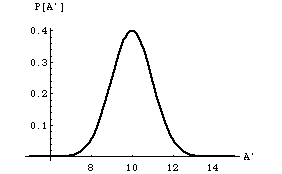
Figure (4)

The following properties follow immediately upon inspection or with some mathematical manipulation.

b. For an experiment where you measure A many times and calculate the average value of all the A's that you record, the theory just developed predicts

c. From the above, you can easily see that the average value of

<A'-> is zero, but if you look at you get

d) Imagine that you measure two independent quantities A and B, each characterized by its own normal distribution function, with different mean values and standard deviations. We call these PA(A') and PB(B') respectively. Imagine you are interested in some new variable Z which is a function of A and B define as G(A,B). The probability density for Z is then given by

If G(A,B) can be approximated by a linear function of A and B in a region centered on the mean values of A and B with extension of the order of their standard deviation it follows that PG(Z) is also a normal distribution centered at G(,) with variance

This is an often quoted formula for the propagation of errors.

We are not yet finished with developing the model. Imagine we perform an experiment in which we make N measurements of A. Our probability distribution P(A') will tell us the average number of times we will measure a number between A' and A'+dA' , which is just NP(A')dA'. Is this what we actually measure in our experiment? No! We only expect to get this result on the average. In any given experiment the number of measurements that result in values between A' and A'+dA' will generally be either greater or smaller than NP(A')dA'. Figure(5) shows graphically what we mean.

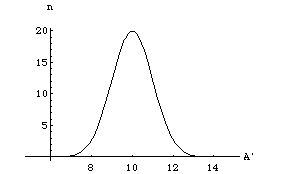
Figure(5)

Our next task is to develop a prediction for the probability for a fluctuation from the value predicted by NP(A')dA' in any given experiment consisting of N measurements. Since P(A') is the probability (density) of a fluctuation from A you can see why this section of the notes is called the average fluctuation of a fluctuation, and that is what we'll calculate right now.

The method we will use is quite useful in other applications so it's worth paying close attention. Consider again an experiment that consists of N measurements. We repeat that on the average NP(A')dA' will yield the number of measurements that give a value between A' and A'+dA'. Now for this to be true we must have obviously picked an interval dA' small enough that P(A') hardly varies within it. In fact let's assume P(A') is constant in dA'. Now we break up the interval dA' into t equal sub-intervals of width dA'/t. Now the probability of one of the measurements in our experiment falling within a particular one of these dA'/t sub-intervals must be P(A')dA'/t which we call p. The probability that it does not fall in a particular interval must simply be 1-p which we call q.

Now here's the important part. The probability of n measurements yielding a value within the original interval dA' must be the sum of the probabilities for all the different ways n values within dA' can be distributed in the t sub-intervals there. Lets take a concrete example. Let the average number of measurements, , predicted to give A' in the interval dA' be 3 and let's calculate the probability that no measurements will actually yield a value in this interval for our experiment. Divide dA' into t=100 parts. We want to pick a large enough value for t such that only two possibilities have any significant chance of happening. Either none of the measurements give a value in a dA' interval or one does. We explicitly want to be able to neglect the possibility that 2 or more measurements might fall into our sub-interval. This can be achieved by making the interval sufficiently small, in other words t must be large.

So take t=100. The probability of a measured value coming in a sub-interval is p=.03 and the probability for one not to be in the sub-interval is q=1-p=0.97. The probability of no value occurring in the 100 sub-intervals must be the product of all hundred sub-interval probabilities, i.e., q100=(.97)100=.048.

How about the probability of one measured value occurring in the 100 intervals. One way this can happen is if the value occurs in the first interval and then not again in the next ninety nine. The probability for this is the product of one p=.03 with ninety nine q=.97's or (.03)1(.97)99=.00147. But wait, there are ninety nine other ways we can get one value in our hundred sub-intervals. It could occur in the second , third, or fourth etc. So we must add all one hundred of these up to give 100(.00147)=.147

Now lets get a general formula based on the p's and q's. For every sub-interval that contains a measurement we will have a factor p, multiplied by a factor q for every sub-interval with no measurement. Remember that p=/t. If we want the probability of n measurements falling in the interval dA' this gives pnqn-t for t sub intervals. Now we need to multiply this by the number of distinct ways of distributing our n measurements among the t sub-intervals. There are t possibilities for the interval the first measurement might be in, t-1 for the second, etc. until the last (or nth) measurement which will has t-n+1. This gives a total of

possibilities. But this counts every different ordering of our n measurements in the same intervals as distinct which they are not. The number of ways or ordering n things is n! and hence we must divide (t-n+1)!=(t)!/(t-n)! by n!. Putting everything together gives the probability of n measurements falling within dA' as

Now t must be chosen much larger than so there will be a negligible chance of getting two or more measurements in a sub-interval. If we let t-> infinity while n stays constant t!/(t-n)! -> tn and if we use the fact that p=/t, and q=1-p we have

We have finally arrived at the celebrated formula due to, and named after, Poisson. It tells us the probability of obtaining n successful outcomes in a random process that on the average would give successful outcomes. In our current application a successful outcome constitutes a measurement that gives a value within dA'. (You might like to try and calculate on the example we used to get started on this journey with =3 but now using the Poisson formula. You will find slight differences. Can you guess why? Consider the value of t that was used.)

The Poisson distribution has a number of very interesting properties.

a. It is normalized in the sense that .

b. It predicts a mean value for n of

c. And a mean value for <(n-<n>)2> of

Thus the standard deviation of the Poisson distribution is just .

Q(n) is plotted for the first ten integer values of and is shown in figure (6).

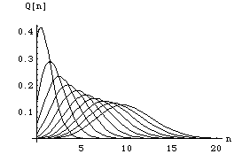
Figure(6)

For =10 the distribution looks a lot like our normal distribution! In fact you should be able to use Stirling's approximation which reads

to show that for large

Look how close they are already for =10

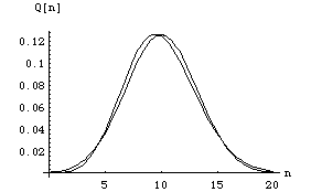
Figure(7)

Now you have all the tools to deal with one of the most common situations in modern experimental physics. It arises because you are trying to determine quantitatively the best value and uncertainty for either a single number or a whole function of one or several variables. Based on a given set of data what is a good strategy on which to proceed?

Let's consider the problem of determining a number first. It would seem that the best way to determine the best guess for the constant we are measuring is to simply take the average of all our measurements. This is true but I would like to suggest an alternative method which provides great power especially when we want to determine functions later.

The new strategy is as follows; from a set of data points that give the values {A'} calculate the variance not from the mean of the {A'} but from some arbitrary test value a. We call this s(a). Now find the value of a that makes this function a minimum and this value provides a best guess for . As you see from the definition of the variance that we are simply minimizing the square errors by adjusting a. Hence the name method of least squares.

This procedure is "justified" theoretically by observing that based on a normal distribution of errors

which on differentiating with respect to a gives zero when a = . You should check that this actually makes a minimum.

clearly the one that minimizes the square error . This is the total probability product of that for each A' i. e.,

This is the view we adopt in the next paragraph.

Now we approach the problem of fitting a function by imagining that we are measuring a lot of different numbers Ai, each of which requires a different experiment. Several attempts at determining a given Ai are made yielding a collection of {Ai'} for each i. One can perform the procedure described above on each of these and determine the best guesses for all the i.

Now assume we have found all the i's in the same way we did for a single number, and we want to predict the probability of getting A'i in an experiment consisting of one measurement at each i. It must be

where

The extension to fitting a function to the data points at each i is now trivial. Set

In which F is to be determined. Obviously the best choice one can make for F is the one that minimizes c2. Generally you will either guess a function or use a function from some theory. The function will have some adjustable parameters in it that you want to choose to get the best agreement with the experimental {A'i}. Choose them to minimize c2. If c2/the number of data points is about 1 you're in good shape. If it's much greater you are in trouble and your guess for F or the theory is not good enough. These issues need to be made more concrete and they can be as we shall see when we discuss confidence limits.